关于lyapunov optimization看了一些资料包括之前看的那一篇论文： infocom2013年的 Profit-Maximizing Virtual Machine Trading in a Federation of Selfish Clouds

Hongxing Li_, Chuan Wu , Zongpeng Li† and Francis C.M. Lau _Department of Computer Science, The University of Hong Kong, Hong Kong, Email: {hxli, cwu, fcmlau}@cs.hku.hk †Department of Computer Science, University of Calgary, Canada, Email: zongpeng@ucalgary.ca

这里做一些摘录和说明：先是wiki上的：前面这里就不紧扯了，就是介绍一下这个方法，大致的意思就是很牛逼，对动态系统有效，队列网络什么的

Lyapunov optimization

From Wikipedia, the free encyclopedia

This article describes Lyapunov optimization for dynamical systems. It gives an example application to optimal control in queueing networks.

## Contents [[hide](http://en.wikipedia.org/wiki/Lyapunov_optimization)] * [1 Introduction](http://en.wikipedia.org/wiki/Lyapunov_optimization#Introduction) * [2 Lyapunov drift for queueing networks](http://en.wikipedia.org/wiki/Lyapunov_optimization#Lyapunov_drift_for_queueing_networks) * [2.1 Quadratic Lyapunov functions](http://en.wikipedia.org/wiki/Lyapunov_optimization#Quadratic_Lyapunov_functions) * [2.2 Bounding the Lyapunov drift](http://en.wikipedia.org/wiki/Lyapunov_optimization#Bounding_the_Lyapunov_drift) * [2.3 A basic Lyapunov drift theorem](http://en.wikipedia.org/wiki/Lyapunov_optimization#A_basic_Lyapunov_drift_theorem) * [3 Lyapunov optimization for queueing networks](http://en.wikipedia.org/wiki/Lyapunov_optimization#Lyapunov_optimization_for_queueing_networks) * [4 Related links](http://en.wikipedia.org/wiki/Lyapunov_optimization#Related_links) * [5 References](http://en.wikipedia.org/wiki/Lyapunov_optimization#References) * [6 Primary Sources](http://en.wikipedia.org/wiki/Lyapunov_optimization#Primary_Sources)

[edit]Introduction

Lyapunov optimization refers to the use of a Lyapunov function to optimally control a dynamical system. Lyapunov functions are used extensively in control theory to ensure different forms of system stability. The state of a system at a particular time is often described by a multi-dimensional vector. A Lyapunov function is a scalar measure of this multi-dimensional state. Typically, the function is defined to grow large when the system moves towards undesirable states. System stability is achieved by taking control actions that make the Lyapunov function drift in the negative direction.

Lyapunov drift is central to the study of optimal control in queueing networks. A typical goal is to stabilize all network queues while optimizing some performance objective, such as minimizing average energy or maximizing average throughput. Minimizing the drift of a quadratic Lyapunov function leads to the backpressure routing algorithm for network stability, also called the max-weight algorithm.^[1] ^[2] Adding a weighted penalty term to the Lyapunov drift and minimizing the sum leads to the drift-plus-penalty algorithm for joint network stability and penalty minimization. ^[3] ^[4] ^[5] The drift-plus-penalty procedure can also be used to compute solutions to convex programs and linear programs.^[6]

[edit]Lyapunov drift for queueing networks

Consider a queueing network that evolves in discrete time with normalized time slots t in {0, 1, 2, …}. Suppose there are N queues in the network, and define the vector of queue backlogs at time t by:

$Q(t) = (Q_1(t), Q_2(t), ..., Q_N(t))$

[edit]Quadratic Lyapunov functions

For each slot t, define L(t) as the sum of the squares of the current queue backlogs (divided by 2 for convenience later):

$L(t) = frac{1}{2}sum_{i=1}^NQ_i(t)^2$

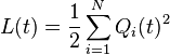
//这里到底是什么玩意完全搞不懂，貌似就是队列积压的工作的数目的平方的和再除以二

This function is a scalar measure of the total queue backlog in the network. It is called quadratic Lyapunov function on the queue state. Define the Lyapunov drift as the change in this function from one slot to the next:

$Delta(t) = L(t+1) - L(t)$ //这里是前后时间片的这样一个函数的差

[edit]Bounding the Lyapunov drift

//貌似小标题是要对李雅普诺夫漂移进行限定

Suppose the queue backlogs change over time according to the following equation:

$Q_i(t+1) = max[Q_i(t) + a_i(t) - b_i(t), 0]$ //单个队列来看，一个队列下一个时间片积累的数目就是收到的减去处理了的（管你怎么处理，直接扔掉也算是处理了）

where a_i(t) and b_i(t) are arrivals and service opportunities, respectively, in queue i on slot t. This equation can be used to compute a bound on the Lyapunov drift for any slot t:

$Q_i(t+1)^2 = max[Q_i(t) + a_i(t) - b_i(t), 0]^2 leq (Q_i(t+1) + a_i(t) - b_i(t))^2$ //这里为什么就要用平方啊，可耻啊，完全搞不懂想干嘛，而且自己推了一下这个不等式尽然不成立

Rearranging this inequality, summing over all i, and dividing by 2 leads to:

$(Eq. 1) text{ } Delta(t) leq B(t) + sum_{i=1}^N Q_i(t)(a_i(t) - b_i(t))$ //如果前面的成立，推出这个不等式，里面的B就是界限之类的东西，但是t+1跑哪里去了？被吃了么？

where B(t) is defined:

$B(t) = frac{1}{2}sum_{i=1}^N[a_i(t)^2 + b_i(t)^2 - 2a_i(t)b_i(t)]$ //上面那个不等式的一部分

Suppose the second moments of arrivals and service in each queue are bounded, so that there is a finite constant B>0 such that for all t and all possible queue vectors Q(t) the following property holds:

$E[B(t) | Q(t)] leq B$ //这个期望中间那一竖搞不清楚是要干嘛，但是大致明白是什么意思了，就是B是这个的上限，因为不管怎么样a(t)-b(t)都是个有限数

Taking conditional expectations of (Eq. 1) leads to the following bound on the conditional expected Lyapunov drift:

$(Eq. 2) text{ } E[Delta(t) | Q(t)] leq B + sum_{i=1}^N Q_i(t)E[a_i(t) - b_i(t) | Q(t)]$ //这里就是替换了一下，中间那一竖还是不知道什么意思

[edit]A basic Lyapunov drift theorem

//这里貌似是基本原理之类的

In many cases, the network can be controlled so that the difference between arrivals and service at each queue satisfies the following property for some real number $epsilon>0$ :

$E[a_i(t) - b_i(t) | Q(t)] leq -epsilon$ //还是进行一些YY，反正就是先YY个上界（其实不是YY，应该是有道理的，使用了某些技术，比如松弛？）

If the above holds for the same epsilon for all queues i, all slots t, and all possible vectors Q(t), then (Eq. 2) reduces to the drift condition used in the following Lyapunov drift theorem. The theorem below can be viewed as a variation on Foster's theorem for Markov chains. However, it does not require a Markov chain structure.

$text{ Theorem (Lyapunov Drift):}$ ^[7] ^[5]

Suppose there are constants 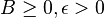$Bgeq 0, epsilon>0$ such that for all t and all possible vectors Q(t) the conditional Lyapunov drift satisfies:

$E[Delta(t)|Q(t)] leq B - epsilon sum_{i=1}^N Q_i(t)$ //上面那个公式继续简化，这样就用两个常量限制了这个不等式

Then for all slots t>0 the time average queue size in the network satisfies:

$frac{1}{t}sum_{tau=0}^{t-1} sum_{i=1}^NE[Q_i(tau)] leq frac{B}{epsilon} + frac{E[L(0)]}{epsilon t}$ //这个公式是下面证明了的，其实就是通过上面一个公式通过一定时间片的累加推出来的一个有意义的结论

$text{ Proof:}$

Taking expectations of both sides of the drift inequality and using the law of iterated expectations yields:

$E[Delta(t)] leq B - epsilon sum_{i=1}^N E[Q_i(t)]$ //这就是上上面那个公式，怎么中间的一竖去掉了，忽悠我呢

Summing the above expression over $tau in {0, 1, ldots, t-1}$ and using the law of telescoping sums gives:

$E[L(t)] - E[L(0)] leq Bt - epsilon sum_{tau=0}^{t-1}sum_{i=1}^NE[Q_i(tau)]$ //来吧从0加到t+1，然后就搞定了 Using the fact that L(t) is non-negative and rearranging the terms in the above expression proves the result.

[edit]Lyapunov optimization for queueing networks

//李雅普诺夫优化之于队列网络

Consider the same queueing network as in the above section. Now define p(t) as a network penalty incurred on slot t. Suppose the goal is to stabilize the queueing network while minimizing the time average of p(t). For example, to stabilize the network while minimizing time average power, p(t) can be defined as the total power incurred by the network on slot t. ^[8] To treat problems of maximizing the time average of some desirable reward r(t), the penalty can be defined p(t) = -r(t). This is useful for maximizing network throughput utility subject to stability. ^[3]

//这里一个比较有用的就是penalty和reward之间可以相互转化，加个负号就行 To stabilize the network while minimizing the time average of p(t), network algorithms can be designed to make control actions that greedily minimize a bound on the following drift-plus-penalty expression on each slot t:^[5]

$Delta(t) + Vp(t)$

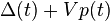
//这里是相当关键的一步，使用的drift-plus-penalty方法，可以简单的理解成使用将这个公式最小化的方法来控制队列

where V is a non-negative weight that is chosen as desired to affect a performance tradeoff. Choosing V = 0 reduces to minimizing a bound on the drift every slot and, for routing in multi-hop queueing networks, reduces to the backpressure routing algorithm developed by Tassiulas and Ephremides.^[1]^[2] Using V>0 and defining p(t) as the network power use on slot t leads to the drift-plus-penalty algorithm for minimizing average power subject to network stability developed by Neely.^[8] Using V>0 and using p(t) as -1 times an admission control utility metric leads to the drift-plus-penalty algorithm for joint flow control and network routing developed by Neely, Modiano, and Li.^[3]

^{//这一段的大致意思就是V=0和V>0是属于不同的情况，讲了一些具体的例子}

A generalization of the Lyapunov drift theorem of the previous section is important in this context. For simplicity of exposition, assume the penalty p(t) is lower bounded by some (possibly negative) real number p_min:

$p(t) geq p_{min} text{ } forall t in {0, 1, 2, ...}$

Let p* represent a desired target for the time average of p(t). Let V be a parameter used to weight the importance of meeting the target. The following theorem shows that if a drift-plus-penalty condition is met, then the time average penalty is at most O(1/V) above the desired target, while average queue size is O(V). The V parameter can be tuned to make time average penalty as close to (or below) the target as desired, with a corresponding queue size tradeoff.

$text{ Theorem (Lyapunov Optimization):}$ ^[5]

Suppose there are constants 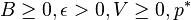$Bgeq 0, epsilon>0, Vgeq 0, p^*$ such that for all t and all possible vectors Q(t) the following drift-plus-penalty condition holds:

![$(Eq. 3) text{ } E[Delta(t) + Vp(t)

Q(t)] leq B + Vp^* - epsilonsum_{i=1}^NQ_i(t)$](http://upload.wikimedia.org/math/b/1/6/b1675c31bb1684bae5ab33afd90e18e3.png)

//这里就是结论了，结合之前bounding的步骤，这里增加了V和p*这两个参数，这样对于一个有penalty需求的动态系统，使用李雅普诺夫优化可以解

Then for all t>0 the time average penalty and time average queue sizes satisfy:

$text{ } frac{1}{t}sum_{tau=0}^{t-1} E[p(tau)] leq p^* + frac{B}{V} + frac{E[L(0)]}{Vt}$
$text{ } frac{1}{t}sum_{tau=0}^{t-1} sum_{i=1}^NE[Q_i(tau)] leq frac{B + V(p^* - p_{min})}{epsilon} + frac{E[L(0)]}{epsilon t}$

//这有两个有用的结论，一个是有关penalty的和队列的时间上平均的大小得到上界

$text{ Proof:}$

//证明就不讲了，和上面那个差不多

Taking expectations of (Eq. 3) and using the law of iterated expectations gives:

$E[Delta(t)] + VE[p(t)] leq B + Vp^* - epsilon sum_{i=1}^NE[Q_i(t)]$

Summing the above over the first t slots and using the law of telescoping sums gives:

$E[L(t)] - E[L(0)] + Vsum_{tau=0}^{t-1}E[p(tau)] leq (B+Vp^*)t - epsilonsum_{tau=0}^{t-1}sum_{i=1}^NE[Q_i(tau)]$

Since L(t) and Q_i(t) are non-negative quantities, it follows that:

$- E[L(0)] + Vsum_{tau=0}^{t-1}E[p(tau)] leq (B+Vp^*)t$

Dividing the above by Vt and rearranging terms proves the time average penalty bound. A similar argument proves the time average queue size bound.

[edit]Related links

[edit]References

^ ^a ^b L. Tassiulas and A. Ephremides, “Stability Properties of Constrained Queueing Systems and Scheduling Policies for Maximum Throughput in Multihop Radio Networks, IEEE Transactions on Automatic Control, vol. 37, no. 12, pp. 1936-1948, Dec. 1992.
^ ^a ^b L. Tassiulas and A. Ephremides, “Dynamic Server Allocation to Parallel Queues with Randomly Varying Connectivity,” IEEE Transactions on Information Theory, vol. 39, no. 2, pp. 466-478, March 1993.
^ ^a ^b ^c M. J. Neely, E. Modiano, and C. Li, “Fairness and Optimal Stochastic Control for Heterogeneous Networks,” Proc. IEEE INFOCOM, March 2005.
[^](http://en.wikipedia.org/wiki/Lyapunov_optimization#cite_ref-now_4-0) L. Georgiadis, M. J. Neely, and L. Tassiulas, “Resource Allocation and Cross-Layer Control in Wireless Networks,” Foundations and Trends in Networking, vol. 1, no. 1, pp. 1-149, 2006.
^ ^a ^b ^c ^d M. J. Neely. Stochastic Network Optimization with Application to Communication and Queueing Systems, Morgan & Claypool, 2010.
[^](http://en.wikipedia.org/wiki/Lyapunov_optimization#cite_ref-neely-dcdis_6-0) M. J. Neely, “Distributed and Secure Computation of Convex Programs over a Network of Connected Processors,” DCDIS Conf, Guelph, Ontario, July, 2005
[^](http://en.wikipedia.org/wiki/Lyapunov_optimization#cite_ref-leonardi_7-0) E. Leonardi, M. Mellia, F. Neri, and M. Ajmone Marsan, “Bounds on Average Delays and Queue Size Averages and Variances in Input-Queued Cell-Based Switches”, Proc. IEEE INFOCOM, 2001.
^ ^a ^b M. J. Neely, “Energy Optimal Control for Time Varying Wireless Networks,” IEEE Transactions on Information Theory, vol. 52, no. 7, pp. 2915-2934, July, 2006.

[edit]Primary Sources

M. J. Neely. Stochastic Network Optimization with Application to Communication and Queueing Systems, Morgan & Claypool, 2010.

Categories:

有关lyapunov optimization的学习笔记哦，original的（第0篇之先看看wiki的解释）

November 26, 2013